Eigenfilter Method for FIR Filter Design #

clear all
close all

%FIGURE LIST

%Figure 1 - Impulse Response
%Figure 2 - Magnitude Response
%Figure 3 - Impulse Response
%Figure 4 - Magnitude Response

f_grid = 12000;
N = 50;
M = ceil(N/2);


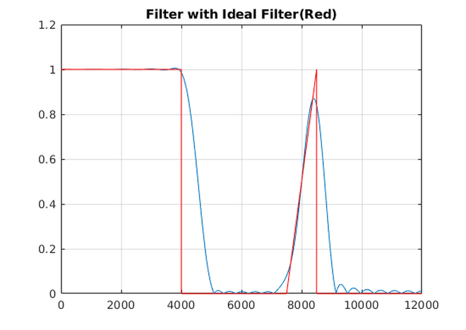
%Example 1: Eigenfilter method used to design a type-1 linear phase FIR filter, N=50. to
%have a magnitude frequency response as close as possible to the desired
%frequency response:
%Fs = 24000 Hz
%0-4000hz - passband, Mag = 1
%5000-7000hz - stop band, Mag = 0;
%7500-8500hz - passband with linear slop, Mag = 1/(8500-7500)
%9000-12000 - stopband, Mag = 0;
Wp = [0 4000 5000 7000 7500 8500 9000 12000];
W  = [1 0 1/(8500-7500) 0]


%build Dw
f2 = linspace(0, 12000, f_grid);
flin= linspace(0,1000,1000);
lin_sec = 1*flin*(1/1000);

Dwtest = []
cnt = 1;
for i = 1:length(f2)
    %less than 4k
    if f2(i) < Wp(2)
        Dwtest = [Dwtest W(1)];
    end

    %transition
    if f2(i) >= Wp(2) & f2(i) <=  Wp(3)
        Dwtest = [Dwtest eps];
    end

    %0
   if (f2(i)) >= Wp(3) & f2(i) <= Wp(4)
       Dwtest = [Dwtest W(2)];
   end

   %tran
   if f2(i) >= Wp(4) & f2(i) <= Wp(5)
       Dwtest = [Dwtest eps];
   end

   %lin
   if f2(i) >= Wp(5) & f2(i) <= Wp(6)
       Dwtest = [Dwtest 1*lin_sec(cnt)];
       cnt = cnt + 1;
   end

   %tran
   if f2(i) >= Wp(6) & f2(i) <= Wp(7)
       Dwtest = [Dwtest eps];
   end

    if f2(i) >= Wp(7) & f2(i) <= Wp(8)
       Dwtest = [Dwtest 0];
   end

end
%Dwtest = ones(1,f_grid);

%f_grid
f = linspace(0,.5,f_grid);
w = 2*pi*f;

%Cw dim = (M+1xfgrid)
Cw = cos(w'*(0:M))';

%Cw M+1x1
%Expand into Cw3 dim = M+1 x M+1 x f_grid
%then trapz over 3rd dimension, w (f_grid) into M+1xM+1
Cw3 = zeros(M+1, M+1, f_grid);
for i = 1:f_grid
    Cw3(:,:,i) = Cw(:,i)*Cw(:,i)';
end

%region to integrate over
%reg = 1:length(Dwtest);
reg = find(Dwtest~=eps);

%build Q
%integrate
Q = trapz(Cw3(:,:,reg),3);
Q = Q + eye(size(Q))*1e-10;

%build P
%Dw 1xf_grid
%Cw(i,:)1 x f_grid
%Ptemp = M+1 x f_grid
Dw = Dwtest;
for i = 1:M+1
    Ptemp(i,:) = Dw.*Cw(i,:);
end


%integrate over w, dim 2
PP= trapz(Ptemp(:,reg),2);
P = PP;

%build d
Dw2 = Dw.^2;
d = trapz(Dw2(reg));

%build Qt
Qt = [Q P;P' d];

%find minimum eigenvector
%A*V = V*D
[V,D] = eigs(Qt,1,'sm');

%build [a0' -1]
%manipulate for ease of building h
a_hat0 = V/(-V(end));
at = a_hat0';
at2 = at(1:length(at)-1);
a_h = .5*at2(2:end);

%build h - filter coefficients
h = [fliplr(a_h) at2(1) (a_h)];


figure
stem(h)
title('Filter Impulse Response')

figure
[h2,w2] = freqz(h);
plot(w2*24000/(2*pi), abs(h2))
title('Filter with Ideal Filter(Red)')
grid on
hold on
plot(f*24000, Dwtest,'color','r')
hold off

%Example 2
%Designing a linear phase type-1 FIR filter with the same frequency response
%as Example 1 with two notches at 4500Hz and 8000Hz
L = 1;
E = zeros(L+3,M+1);
temp = Cw3(:,:,4500);
E(1,:) = temp(1,:);

temp2 = diff(Cw3,1,3);
temp3 = temp2(:,:,4500);
E(2,:) = temp3(1,:);

temp22 = Cw3(:,:,8000);
E(3,:) = temp22(1,:);

temp22 = diff(Cw3,1,3);
temp32 = temp22(:,:,8000);
E(4,:) = temp32(1,:);

B  = null([E zeros(size(E,1),1)]);

n  = B'*Qt*B ;

[V1,e1] = eigs(n, 1,'sm');

ao = B*V1;

ao_hat = ao/(-ao(end));
at2_2 = ao_hat(1:length(ao_hat)-1)';
a_h2 = .5*at2_2(2:end);


%build h
hh1 = [fliplr(a_h2) at2_2(1) (a_h2)];
hh3 = hh1;


figure
stem(hh3)
title('Filter w/ Notches Impulse Response')

figure
[h3,w3] = freqz(hh3);
plot(w3*24000/(2*pi), abs(h3))
title('Filter with Ideal Filter(Red), Notch at 4.5KHz and 8.5KHz')
grid on
hold on
plot(f*24000, Dwtest,'color','r')

hold off