Introduction to Least Mean Square Algorithm with MATALB #
The LMS algorithm, also known as the Widrow-Hoff algorithm, is a widely used adaptive filtering algorithm that is commonly employed in various areas of signal processing, communication systems, and pattern recognition. In this introduction, we will explore the basic concepts and principles of the LMS algorithm.
The LMS algorithm works by iteratively updating its model parameters to minimize the error between predicted and actual outputs. It starts with an initial set of model weights and iteratively updates them based on the gradient of the error with respect to the model weights. The gradient is computed using the instantaneous values of input features and the corresponding target output. The algorithm uses a learning rate (\(\mu\)), which determines the step size of the weight updates, and controls how fast the algorithm adapts to the data.
Smaller learning rates result in slower convergence but can offer more stability, while larger learning rates can lead to faster convergence but may be less stable. The LMS algorithm continues to update the model weights until the error converges to a minimum or a predefined stopping criterion is met. The simplicity of the LMS algorithm lies in its ability to continuously update its model parameters based on the instantaneous error, making it suitable for online and real-time learning scenarios.
The Circuit #
                           ┌───┐ e[n]
u[n]─────────────┬─────────┤ - ├──────────────────────────────────────┐
                 │         └─▲─┘                                      │
                 │  u_hat[n] │                                        │
             ┌───▼───┐       │       ┌───────┐                      * │
             │   -1  │     ┌─┴─┐  *  │   -1  │ w[n]┌───┐   ┌───┐    ┌─▼─┐
             │   Z   │     │ x ◄──┬──┤   Z   ├─────┤ + ◄───┤ x ◄────┤ x │
             │       │     └─▲─┘  │  │       │     └─▲─┘   └─▲─┘    └─▲─┘
             └───┬───┘       │    │  └───────┘       │       │        │
                 │           │    │w[n-1]            │       │        │
                 │           │    └──────────────────┘       mu       │
                 │           │                                        │
          u[n-1] │           │                                        │
                 └───────────┴────────────────────────────────────────┘
The Algorithm #
$$ \hat{u} = u[n-1] \cdot conj(w[n-1]) $$ $$ e[n] = u[n] - \hat{u}[n]$$ $$ w[n] = w[n-1] + \mu \cdot (u[n-1] \cdot conj(e[n])) $$
LMS Applied #
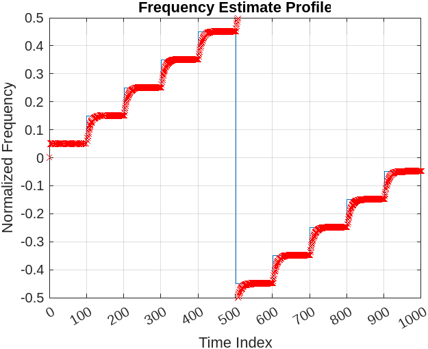
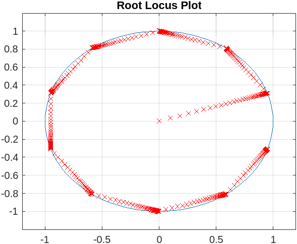
In this article we will apply the LMS to track a single tone in our signal. We will create a time sequence of 10 sinusoids, each 100 samples long. The LMS algorithm will run against all 1,000 clocks and adapt each time the frequency changes.
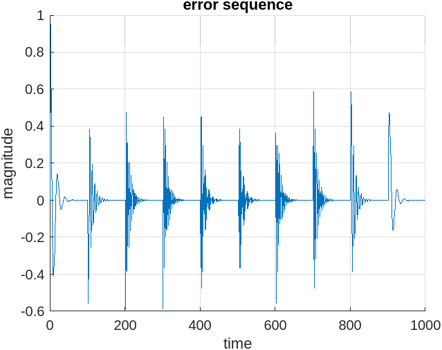
The output of the LMS algorithm, \( e[n]\), will temporarily output error each time the frequency of the tone changes, but in the error plots below you can see the error drive to zero as the weight converges.
Results #


MATLAB Code #
clear all;
close all;

% time_sequence init
% we will create 10 tones, 100 long each
tones = complex(zeros(10,100));

% list of normalized frequencies
f = [.05, .15, .25, .35, .45 , .55, .65, .75, .85, .95];
f(f>.5) = f(f>.5)-1;

% noise
noise_sd0 = .25 + .25*i;
noise_sd01 = .1*rand(10*100,1) + i*.1*rand(10*100,1);

% build time sequence
A = 1;
for n = 1:10
    tones(n,:) = A*exp(j*2*pi*[0:99]*f(n));
end

N = 1024;
figure
for n = 1:10
    subplot(2,5,n)
    plot([-N/2:(N/2 -1)]/N, fftshift(abs(fft(tones(n,:), N))/100))
    grid on
    axis([-.5 .5 0 1])
    titstr = sprintf('Frequency = %f', f(n));
    ylabel('Mag')
    xlabel('Normalized Frequency')
    title(titstr)
end

figure
N= 2^14;
u = reshape(tones',1,size(tones,1)*size(tones,2));
plot([-N/2:(N/2 -1)]/N, fftshift(abs(fft(u, N))/100))
axis([-.5 .5 0 1])
xlabel('Mag')
ylabel('Normalized Frequency')
title('whole sequence spectrum')
set(gca, 'YTick', [0:.5:1])
set(gca, 'XTick', [-.5:.1:.5])
grid on


%% LMS algorithm

% try different mu's
mu    = 0.1;
ww    = complex(zeros(1,1))';
w(n-1)= rand;
for n = 2:length(u)
    u_hat(n)   = u(n-1) *conj(w(n-1));
    e(n)       = u(n) - u_hat(n);
    w(n)       = w(n-1) + mu * (u(n-1) * conj(e(n)));
end


f_stairs = ones(1,10*100);
q=1;
cnt=1;
for indx = 1:10*100
    f_stairs(indx) = f_stairs(indx)*f(q);
    if(mod(indx,100) == 0)
        q = q+1;
    end

end

%% stairscase plot of frequency estimation
figure
stairs(f_stairs)
for n = 1:length(w)
    hold on
    plot(n, angle(w(n))/(2*pi),'rx')
    hold off
end
ylabel('Normalized Frequency')
xlabel('Time Index')
title('Frequency Estimate Profile')
grid on
set(gca, 'YTick', [-.5:.1:.5])
set(gca, 'XTick', [0:100:1000])

%% Plot
figure
plot(exp(j*2*pi*(0:0.01:1)))
hold on
for n = 1:length(w)
   plot(real(roots([1 -w(n) ])), imag(roots([1 -w(n) ])),'rx')
end
hold off
grid on
axis([-1.2 1.2 -1.2 1.2])
set(gca, 'YTick', [-1:.2:1])
set(gca, 'XTick', [-1:.5:1])
title('Root Locus Plot')

%%
figure
hold on
plot(real(e))
title('error sequence')
grid on
ylabel('magnitude')
xlabel('time')